1. What is DBMS? Advantages and Disadvantages of DBMS over File System. Difference between DBMS and File System

DBMS (Database Management System) is software that allows creation, definition, manipulation, and management of data in a database. It acts as an interface between the user/application and the physical database, providing controlled access (storage, retrieval, update, security) to data.

Advantages of DBMS over File System

• Data redundancy and inconsistency: Redundancy is the concept of repetition of data i.e. each data may have more than a single copy. The file system cannot control the redundancy of data as each user defines and maintains the needed files for a specific application to run. There may be a possibility that two users are maintaining the data of the same file for different applications. Hence changes made by one user do not reflect in files used by second users, which leads to inconsistency of data. Whereas DBMS controls redundancy by maintaining a single repository of data that is defined once and is accessed by many users. As there is no or less redundancy, data remains consistent.

• Data sharing: The file system does not allow sharing of data or sharing is too complex. Whereas in DBMS, data can be shared easily due to a centralized system.

• Data concurrency: Concurrent access to data means more than one user is accessing the same data at the same time. Anomalies occur when changes made by one user get lost because of changes made by another user. The file system does not provide any procedure to stop anomalies. Whereas DBMS provides a locking system to stop anomalies to occur.

• Data searching: For every search operation performed on the file system, a different application program has to be written. While DBMS provides inbuilt searching operations. The user only has to write a small query to retrieve data from the database.

• Data integrity: There may be cases when some constraints need to be applied to the data before inserting it into the database. The file system does not provide any procedure to check these constraints automatically. Whereas DBMS maintains data integrity by enforcing user-defined constraints on data by itself.

• System crashing: In some cases, systems might have crashed due to various reasons. It is a bane in the case of file systems because once the system crashes, there will be no recovery of the data that's been lost. A DBMS will have the recovery manager which retrieves the data making it another advantage over file systems.

• Data security: A file system provides a password mechanism to protect the database but how long can the password be protected? No one can guarantee that. This doesn't happen in the case of DBMS. DBMS has specialized features that help provide shielding to its data.

• Backup: It creates a backup subsystem to restore the data if required.

• Interfaces : It provides different multiple user interfaces like graphical user interface and application program interface.

• Easy Maintenance : It is easily maintainable due to its centralized nature.

Disadvantages of DBMS

1. High cost of software, hardware, and skilled personnel (DBA).

2. Complexity of design and administration.

3. Increased overhead (CPU, memory) compared to simple file processing.

4. Vulnerability — a single point of failure if not properly backed up.

5. Conversion/migration cost from existing file systems.

Difference between DBMS and File System

Basis	File System	DBMS
Redundancy	High redundancy	Redundancy controlled/minimized
Data Sharing	Difficult	Easy, multi-user
Data Integrity	Not enforced	Enforced via constraints
Security	Limited	Strong, multi-level
Backup/Recovery	Manual, weak	Automatic, robust
Query Capability	No query language	Powerful query languages (SQL)
Data Independence	Not present	Present (logical & physical)
Concurrency	Not handled well	Handled via locking/transactions
Cost	Low	High

---

2. Three-Layer (Three-Schema) Architecture of DBMS, Schema, Logical and Physical Independence

The 3-Tier Architecture is one of the most popular and effective architectural models in the design and development of modern database-driven applications. It is widely used in Database Management Systems (DBMS) for organizing and managing complex data interactions across various layers of an application. Whether you're building a scalable enterprise application or a responsive web service, understanding 3-Tier Architecture is crucial for efficient system design and management.

In this article, we will explain the details of the 3-Tier Architecture in DBMS, explaining each of its components, the role it plays in application development, and the key benefits it offers for building robust, secure, and maintainable systems.

What is 3 Tier Architecture in DBMS?

In DBMS, the 3-tier architecture is a client-server architecture that separates the user interface, application processing, and data management into three distinct tiers or layers. The 3-tier architecture is widely used in modern web applications and enterprise systems because it offers scalability, flexibility, and security. Here is a brief description of each tier in the 3-tier architecture:

• Presentation Tier (User Interface Layer)

• Application Tier (Business Logic Layer)

• Data Management Tier (Database Layer)

This separation of concerns allows for easier maintenance, scalability, and flexibility in system design, enabling developers to work independently on each layer without disturbing the others.

Components of the 3-Tier Architecture

1. Presentation Tier (User Interface Layer)

The presentation tier is the user interface or client layer of the application. It is responsible for presenting data to the user and receiving input from the user. This tier communicates with the Application Tier to process user requests and display relevant information. This tier can be a web browser, mobile app, or desktop application

• What It Does: It ensures the application is user-friendly by providing interfaces such as web browsers, mobile apps, or desktop applications.

• Example: If you’re using a banking app, the presentation tier would display your account balance, allow you to make transfers, and display results based on your actions.

Why it is Important?

• The Presentation Layer focuses purely on the user interface, ensuring smooth interactions and enhancing user experience (UX).

• It abstracts the business logic and data management complexities, making the system more user-friendly.

2. Application Tier ( Business Logic Layer)

The application tier is the middle layer of the 3-tier architecture. It acts as the intermediary between the Presentation Tier and the Data Management Tier. It is responsible for processing and managing the business logic of the application. This tier communicates with the presentation tier to receive user input and communicates with the data management tier to retrieve or store data. This tier may include application servers, web servers, or APIs.

• What It Does: It houses the application's core functionality, such as calculating values, applying rules, handling workflows, etc.

• Example: If you're purchasing an item through an e-commerce platform, the Application Layer handles all the logic like verifying available stock, applying discounts, calculating taxes, and confirming your payment method.

Why is it Important?

• It decouples the core business logic from the user interface, making it easier to change or update business rules without affecting the user-facing part of the application.

• This tier allows for better management of application workflows and business decisions

3. Data Management Tier ( Database Layer)

The Data Management tier is the bottom layer of the 3-tier architecture. It is responsible for managing and storing data. This tier can include databases, data warehouses, or any other persistent data storage solution. The data management tier communicates with the application tier save, retrieve, or manipulate data according to the business logic.

• What It Does: It ensures that the data is safely stored, retrieved, and maintained. It handles the database connections and ensures data integrity.

• Example: In a customer relationship management (CRM) system, this tier would store customer details, transaction history, and other data relevant to the business.

Why is it Important?

• This layer ensures data consistency, security, and integrity. By abstracting the database layer from the application logic, it allows developers to modify database structures without impacting the overall application functionality.

• It is also where optimizations like indexing, data replication, and data security are handled.

Why Choose 3-Tier Architecture?

The 3-tier architecture in DBMS provides several advantages for developers and organizations working on large-scale, database-driven applications. Here are a few key benefits:

1. Scalability: The separation of the three tiers allows each layer to scale independently. For instance, if the number of users increases, you can scale the Presentation Tier by adding more web servers, or you can enhance the Data Management Tier by optimizing or adding additional databases without affecting the Application Tier.

2. Flexibility: Each layer is loosely coupled, meaning you can modify or upgrade any of the layers without disrupting the others. For example, you could swap out the database system in the Data Management Tier (e.g., from MySQL to PostgreSQL) without affecting the business logic or user interface layers.

3. Security: By isolating the Data Management Tier, you can enforce better security practices, such as restricting direct access to the database and protecting sensitive data. The Presentation Tier and Application Tier interact via secure APIs or middleware, reducing the risk of unauthorized access.

4. Maintainability: Because the architecture is modular, it’s easier to maintain and update. If you need to change the user interface or tweak the business logic, these changes won’t require touching the underlying data storage or database. The separation of concerns also means that developers can specialize in one of the layers (frontend, backend, or database), allowing for more focused development and faster updates.

5. Improved Performance: The layered approach improves system performance by ensuring that each tier is optimized for its specific function. For instance, database queries in the Data Management Tier can be optimized independently, and the Application Tier can focus on processing requests efficiently.

3-Tier Schema Architecture in DBMS

In DBMS, the 3-Tier Schema Architecture refers to how the data is logically and physically organized in three layers:

1. Physical Level At the physical level, the information about the location of database objects in the data store is kept. Various users of DBMS are unaware of the locations of these objects.In simple terms,physical level of a database describes how the data is being stored in secondary storage devices like disks and tapes and also gives insights on additional storage details.

2. Conceptual Level At conceptual level, data is represented in the form of various database tables. For Example, STUDENT database may contain STUDENT and COURSE tables which will be visible to users but users are unaware of their storage.Also referred as logical schema,it describes what kind of data is to be stored in the database.

3. External Level An external level specifies a view of the data in terms of conceptual level tables. Each external level view is used to cater to the needs of a particular category of users. For Example, FACULTY of a university is interested in looking course details of students, STUDENTS are interested in looking at all details related to academics, accounts, courses and hostel details as well. So, different views can be generated for different users. The main focus of external level is data abstraction.

Conclusion :

In conclusion, a Database Management System (DBMS) employs the 3-Tier Architecture, a tried-and-true structure that separates an application into three main layers: Presentation, Application Logic, and Data. This architectural technique is increasingly popular for creating dependable and maintainable software systems that communicate with databases because it improves the modularity, scalability, security, reusability, and flexibility of applications.

Difference

Basis	Logical Data Independence	Physical Data Independence
Definition	Conceptual schema changes don't affect external schema	Internal schema changes don't affect conceptual schema
Difficulty	Difficult to achieve	Easy to achieve
Example	Adding a new table/attribute	Changing storage device or file structure

---

3. What is DBA? Applications/Responsibilities of DBA

A Database Administrator (DBA) is a person responsible for managing and maintaining a Database Management System (DBMS) to ensures the database runs smoothly, securely, and efficiently.The DBA handles task include database installation, configuration, security management, user authorization, performance monitoring, backup, and recovery. And also responsible for handling capacity planning, troubleshooting, migration, and system upgrades.Overall, a DBA ensures that the database remains secure, available, consistent, and reliable for the organization.

Types of Database Administrator (DBA)

There are different types of Database Administrators (DBAs) based on their roles and responsibilities in managing, maintaining, and securing database systems.

• Administrative DBA – Manages the database server, backups, security, replication, migration, and troubleshooting to keep the system running properly.

• Data Warehouse DBA – Designs and maintains the data warehouse, integrates data from multiple sources, and performs data cleaning before loading.

• Cloud DBA – Manages databases hosted on cloud platforms, ensuring data security, availability, scalability, and reduced risk of data loss.

• Development DBA – Develops queries, stored procedures, and database code to support application and organizational requirements.

• Application DBA – Manages database components related to applications, including installation, upgrades, cloning, and data load processes.

• Database Architect – Designs database schemas, tables, and overall structure based on organizational needs.

• OLAP DBA – Designs and maintains multidimensional cubes for OLAP and decision-support systems.

• Data Modeler – Designs data models and structures; often supports database architecture but may not always be classified as a DBA.

• Task-Oriented DBA – Specializes in specific tasks such as backup and recovery, usually found in large organizations.

• Database Analyst – Assists in database design and analysis; sometimes considered a junior DBA or similar to a data architect role depending on the organization.

Importance of Database Administrator (DBA)

• Manages and control all three levels of DBMS architecture—internal, conceptual, and external levels.

• The DBA defines the overall structure of the database and provides different views for users and applications.

• They are responsible for maintaining data integrity, security, and access control, ensuring that only authorized users can access the database.

• The DBA also manages user profiles, protects the system from unauthorized access, and minimizes the risk of data loss through regular backup and recovery procedures.

Duties of Database Administrator (DBA)

• Hardware Selection – Chooses cost-effective and efficient hardware suitable for organizational needs.

• Data Integrity and Security Management – Ensures data accuracy, maintains relationships between data, and protects the database from unauthorized access.

• Database Accessibility Control – Grants user permissions and manages access rights to control who can view or modify data.

• Database Design – Responsible for logical design, physical design, external model design, and enforcing integrity and security constraints.

• Database Implementation – Installs and configures the DBMS and supervises database creation and data loading.

• Query Processing Optimization – Improves query execution speed, performance, and accuracy.

• Performance Tuning – Tunes SQL queries and optimizes the database system to ensure fast and reliable data access.

---

Summary :

DBA (Database Administrator) is the person (or team) responsible for the overall control, management, and maintenance of the DBMS and the database(s).

Responsibilities / Applications of DBA

1. Schema definition – creating the original database schema.

2. Storage structure and access method definition.

3. Schema and physical organization modification – as requirements change.

4. Granting authorization for data access – managing user permissions/roles.

5. Routine maintenance – backup, recovery planning, periodic upgrades.

6. Ensuring data security and integrity.

7. Performance monitoring and tuning – indexing, query optimization.

8. Capacity planning – managing storage growth.

9. Liaison with users – understanding requirements, training users.

10. Concurrency control management.

---

4. Attributes, Domain, Cardinality, Keys

Attributes

An Attribute is a property or characteristic that describes an entity in a database. It provides specific information used to identify, categorize, and manage entities effectively. Without attributes, entities have no meaningful data.

For example:

• Let's take the student as an entity. Students will have multiple attributes such as roll number, name, and class.

• These attributes are used to describe the student in more detail.

• As shown in the figure, roll_no, name, and class are the attributes of the entity Student.

• All three attributes give meaning to the entity. The information about the student entity lies in all 3 attributes.

Domain :

• Data is modeled by using atomic values as the basis for the domain. In the relational model, atomic values refer to the number of values in a domain that are indivisible. First Name is a set of character strings that represent the names of people in the domain.

• In a database, a domain is a column that contains a data type. Data types can be built-in (such as integers or strings) or custom types that define constraints on the data themselves.

• A SQL Domain is a set of valid values that can be named by the user. Name of the Domain’s set of values that must belong to (for character string types). This is the name of the domain’s default Collation.

Example :

In a table, a domain is a set of values that can be used to attribute an attribute. The domain of a month can accept January, February, etc. A domain of integers can accept whole numbers that are negative, positive, and zero in December.

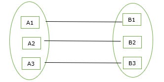
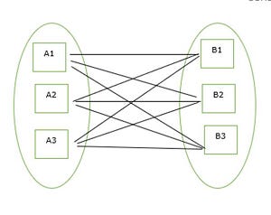
Cardinality :

In the view of databases, cardinality refers to the uniqueness of data values that are contained in a column. High cardinality is nothing but the column contains a large percentage of totally unique values. Low cardinality is nothing but the column which has a lot of “repeats” in its data range.

Cardinality between the tables can be of type one-to-one, many-to-one or many-to-many.

Mapping Cardinality

It is expressed as the number of entities to which another entity can be associated via a relationship set.

For binary relationship set there are entity set A and B then the mapping cardinality can be one of the following −

• One-to-one

• One-to-many

• Many-to-one

• Many-to-many

One-to-one relationship

One entity of A is associated with one entity of B.

Example

Given below is an example of the one-to-one relationship in the mapping cardinality. Here, one department has one head of the department (HOD).

One-to-many relationship

An entity set A is associated with any number of entities in B with a possibility of zero and entity in B is associated with at most one entity in A

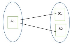
Example

Given below is an example of the one-to-many relationship in the mapping cardinality. Here, one department has many faculties.

Many-to-one relationship

An entity set A is associated with at most one entity in B and an entity set in B can be associated with any number of entities in A with a possibility of zero.

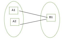
Example

Given below is an example of the many-to-one relationship in the mapping cardinality. Here, many faculties work in one department.

Many-to-many relationship

Many entities of A are associated with many entities of B.

An entity in A is associated with many entities of B and an entity in B is associated with many entities of A.

Many to many=many to one + one to many

Example

Given below is an example of the many-to-many relationship in the mapping cardinality. Here, many employees work on many projects.

Keys in Relational Model

Keys are fundamental elements of the relational database model that ensure uniqueness, data integrity, and efficient data access.

• They uniquely identify each row in a table.

• They prevent data duplication and maintain consistency.

• They create relationships between different tables.

Importance of Keys in DBMS

• Uniqueness: Keys ensure that each record in a table is unique and can be identified distinctly.

• Data Integrity: Keys prevent data duplication and maintain the consistency of the data.

• Efficient Data Retrieval: Keys help in creating relationships between tables, allowing faster queries and better data organization.

• Without keys, managing large databases would become difficult, and data retrieval would be slow and error-prone.

Types of Database Keys

1. Candidate Key

The minimal set of attributes that can uniquely identify a tuple is known as a candidate key. For Example, STUD_NO in STUDENT relation.

• A candidate key is a minimal super key with no redundant attributes.

• It must contain unique values, ensuring that no two rows have the same value in the candidate key’s columns.

• Every table must have at least a single candidate key.

• A table can have multiple candidate keys but only one primary key.

Example: For the STUDENT table below, STUD_NO can be a candidate key, as it uniquely identifies each record.

Table: STUDENT_COURSE

A composite candidate key example: {STUD_NO, COURSE_NO} can be a candidate key for a STUDENT_COURSE table.

2.Super Key:

The set of one or more attributes (columns) that can uniquely identify a tuple (record) is known as Super Key. It may include extra attributes that aren't important for uniqueness but still uniquely identify the row. For Example, STUD_NO, (STUD_NO, STUD_NAME), etc.

• A super key can contain extra attributes that aren’t necessary for uniqueness.

• For example, if the "STUD_NO" column can uniquely identify a student, adding "SNAME" to it will still form a valid super key, though it's unnecessary.

Example: Consider the STUDENT table

A super key could be a combination of STUD_NO and PHONE, as this combination uniquely identifies a student.

3. Alternate Key

An alternate key is any candidate key in a table that is not chosen as the primary key. In other words, all the keys that are not selected as the primary key are considered alternate keys.

• An alternate key is also referred to as a secondary key because it can uniquely identify records in a table, just like the primary key.

• An alternate key can consist of one or more columns (fields) that can uniquely identify a record, but it is not the primary key

Example: In the STUDENT table, both STUD_NO and PHONE are candidate keys. If STUD_NO is chosen as the primary key, then PHONE would be considered an alternate key.

4. Foreign Key

A foreign key is an attribute in one table that refers to the primary key in another table. The table that contains the foreign key is called the referencing table and the table that is referenced is called the referenced table.

• A foreign key in one table points to the primary key in another table, establishing a relationship between them.

• It helps connect two or more tables, enabling you to create relationships between them. This is important for maintaining data integrity and preventing data redundancy.

• They act as a cross-reference between the tables.

Example: Consider the STUDENT_COURSE table

• STUD_NO in the STUDENT_COURSE table is a foreign key that refers to the STUD_NO primary key of the STUDENT table.

• Unlike a primary key, a foreign key can contain duplicate values and may be NULL. For example, STUD_NO appears multiple times in STUDENT_COURSE because a student can enroll in more than one course.

• However, STUD_NO in the STUDENT table is a primary key, so it must always be unique and non-NULL.

5. Partial Key

A partial key is chosen from a weak entity to help identify records, but it cannot uniquely identify a record by itself.

• Helps distinguish records in a weak entity when combined with data from a related strong entity.

• It cannot be NULL, as it is needed to identify records with other data.

• It can be a single column or a combination of columns.

• Ensures consistency when paired with data from a strong entity.

Example: In a STUDENT_COURSE table, the combination of STUD_NO and COURSE_CODE can be a partial key.

6. Primary Key

A primary key is chosen from the set of candidate keys to uniquely identify each record in a table. For example, in the STUDENT table, both STUD_NO and STUD_PHONE can be candidate keys, but STUD_NO is selected as the primary key.

• It cannot be NULL, as each record must have a valid identifier.

• It may be single-column or composite (made of multiple columns).

• Databases often organize data using the primary key to allow faster access and searching.

Example: The STUDENT table has the structure Student(STUD_NO, SNAME, ADDRESS, PHONE), where STUD_NO is the primary key.

7. Secondary Key :

A Secondary Key is an attribute or a combination of attributes used to search or query records in a table, but it doesn’t guarantee uniqueness.

• It helps in retrieving data quickly, often by creating indexes.

• It doesn’t uniquely identify each record; multiple records can have the same value.

• For example, STUD_NAME in a STUDENT table can be used to find students by name, even though many students may share the same name.

• It’s mainly for improving search efficiency, not for maintaining data uniqueness.

Here's an example of how the STUDENT table might look with STUD_NAME as a secondary key:

8. Unique Key:

A Unique Key is a database constraint that ensures that all values in a specific column or a combination of columns are unique across all the rows in a table. It guarantees that no two rows in the table can have the same value in the columns defined as part of the unique key.

• Prevents duplicate values in the specified column(s).

• It allows NULL values, but only one NULL per column.

• It can be applied to a single column or multiple columns.

• Helps maintain the integrity and accuracy of the data in the table.

Example: In the STUDENT_COURSE table, the combination of STUD_EMAIL and STUD_NAME can form a Unique Key to ensure that each student’s email and name pair is unique across the table.

9. Composite Key:

Sometimes, a single column is not enough to uniquely identify all records in a table, so a combination of multiple attributes is used. An optimal set of such attributes is chosen to ensure that every row is uniquely identifiable

It acts as a primary key if there is no primary key in a table

• Two or more attributes are used together to make a composite key .

• Different combinations of attributes may give different accuracy in terms of identifying the rows uniquely.

Example: In the STUDENT_COURSE table, {STUD_NO, COURSE_NO} can form a composite key to uniquely identify each record.

10. Surrogate Keys:

A surrogate key is an artificial attribute created to uniquely identify each record in a table when no suitable natural key is available.

• It is usually generated automatically by the system (like auto-increment numbers).

• It acts as a primary key when natural or composite keys are not practical or efficient.

• A single system-generated attribute is used to make a surrogate key.

• It does not have any real-world meaning and is used only for identification purposes.

Example: STUDENT_ID is used as a surrogate key to uniquely identify each record in the STUDENT_COURSE table, without relying on natural attributes like name or email.

---

Summary

Attribute

An attribute is a property or characteristic of an entity (e.g., Name, Age, RollNo of a Student entity). Represented as columns in a table.

i) Composite Attribute An attribute that can be divided into smaller sub-parts, each representing a more basic attribute with independent meaning.

• Example: Address → Street, City, State, Pincode. Name → First Name, Last Name.

ii) Multivalued Attribute An attribute that can hold multiple values for a single entity instance.

• Example: A person can have multiple Phone Numbers or multiple Email IDs. Represented with double ellipse in ER diagrams.

iii) Derived Attribute An attribute whose value can be calculated/derived from other attributes; not stored directly.

• Example: Age can be derived from Date of Birth; Total Marks derived from individual subject marks. Represented with dashed ellipse.

Domain

The domain of an attribute is the set of all permissible/legal values that attribute can take.

• Example: domain of Age = positive integers (0–120); domain of Gender = {Male, Female, Other}.

Cardinality

Cardinality defines the number of times an entity of one entity set can be associated with an entity of another entity set in a relationship.

Types of Cardinality (Mapping Cardinality):

1. One-to-One (1:1) – one entity in A relates to exactly one entity in B. E.g., Person – Passport.

2. One-to-Many (1:N) – one entity in A relates to many entities in B. E.g., Department – Employees.

3. Many-to-One (N:1) – many entities in A relate to one entity in B. E.g., Students – School.

4. Many-to-Many (M:N) – many entities in A relate to many entities in B. E.g., Students – Courses.

Key

A key is an attribute or set of attributes used to uniquely identify a tuple (row) in a relation.

• Super Key: A set of one or more attributes that can uniquely identify a tuple. May contain extra attributes that are not necessary for uniqueness.

  • Example: {RollNo}, {RollNo, Name} are both super keys.

• Candidate Key: A minimal super key — i.e., a super key with no redundant attribute; removing any attribute breaks uniqueness.

  • Example: {RollNo}, {Email} (if both uniquely identify students).

• Primary Key: A candidate key chosen by the designer to uniquely identify tuples in a table. Cannot have NULL values; only one primary key per table.

• Foreign Key: An attribute (or set of attributes) in one table that refers to the primary key of another (or same) table, used to maintain referential integrity between two tables.

---

Important: "Minimal Candidate Key is Super Key" — Explanation

• A super key is any combination of attributes that uniquely identifies a tuple (uniqueness is the only requirement; may have extra/redundant attributes).

• A candidate key is a super key that is minimal — meaning no proper subset of it is also a super key (no redundant attribute).

• Hence, every candidate key is, by definition, a super key (since it satisfies the uniqueness property), but it is the smallest/minimal such set.

• Formally: Candidate Key = Minimal Super Key.

• Example: In Student(RollNo, Name, Email, Phone):

  • Super keys: {RollNo}, {RollNo, Name}, {RollNo, Email}, {Email}, {Email, Phone}, ...

  • Candidate keys: {RollNo}, {Email} — both are minimal (cannot remove any attribute and still be unique), so both are super keys too.

  • {RollNo, Name} is a super key but NOT a candidate key because RollNo alone is already sufficient (Name is redundant).

So: All candidate keys are super keys, but not all super keys are candidate keys (the reverse is not true) — because super keys may have unnecessary extra attributes.

---

5. Relational Algebra

Relational Algebra is a procedural query language consisting of a set of operations that take one or two relations as input and produce a new relation as output. It is the theoretical foundation for SQL.

a) Select (σ)

1. Selection(σ)

The Selection Operation is basically used to filter out rows from a given table based on certain given condition. It basically allows us to retrieve only those rows that match the condition as percondition passed during SQL Query.

Example: If we have a relation R with attributes A, B, and C, and we want to select tuples where C > 3, we write:

A	B	C
1	2	4
2	2	3
3	2	3
4	3	4

σ(c>3)(R) will select the tuples which have c more than 3.

Output:

A	B	C
1	2	4
4	3	4

Explanation: The selection operation only filters rows but does not display or change their order. The projection operator is used for displaying specific columns.`

b) Project (π)

Project operation selects (or chooses) certain attributes discarding other attributes. The Project operation is also known as vertical partitioning since it partitions the relation or table vertically discarding other columns or attributes. Notation:

πA(R)

where 'A' is the attribute list, it is the desired set of attributes from the attributes of relation(R), symbol 'π(pi)' is used to denote the Project operator, R is generally a relational algebra expression, which results in a relation. Example -

πAge(Student)

πDept, Sex(Emp)

Example - Given a relation Faculty (Class, Dept, Position) with the following tuples:

Class Dept Position

5 CSE Assistant Professor

5 CSE Assistant Professor

6 EE Assistant Professor

6 EE Assistant Professor

1. Project Class and Dept from Faculty -

πClass, Dept(Faculty)

Class Dept

5 CSE

6 EE

Here, we can observe that the degree (number of attributes) of resulting relation is 2, whereas the degree of Faculty relation is 3, So from this we can conclude that we may get a relation with varying degree on applying Project operation on a relation. Hence, the degree of resulting relation is equal to the number of attribute in the attribute list 'A'

c) Left Outer Join (⟕)

Returns all tuples from the left relation, and matching tuples from the right relation; unmatched right-side attributes are filled with NULL.

R ⟕ S

d) Natural Join (⋈)

A join that combines two relations based on all common attribute names, with equality condition, and removes duplicate columns automatically.

R ⋈ S

e) Self Join

A join of a relation with itself, typically used to compare tuples within the same relation (e.g., finding employees and their managers in the same Employee table). Achieved using aliasing (renaming) since SQL/relational algebra requires distinct relation names.

f) Theta Join (⋈θ)

A join that combines tuples from two relations based on a general condition (θ), which can use any comparison operator (=, <, >, ≤, ≥, ≠), not just equality.

R ⋈θ S    e.g., R ⋈ R.a > S.b S

g) Rename (ρ)

Renames a relation and/or its attributes, useful for self-joins and clarity.

ρ NewName (Relation)
ρ NewName(A1,A2,...) (Relation)

h) Full Outer Join (⟗)

Returns all tuples from both relations; unmatched tuples from either side are padded with NULL.

R ⟗ S

i) Right Outer Join (⟖)

Returns all tuples from the right relation, and matching tuples from the left; unmatched left-side attributes filled with NULL.

R ⟖ S

j) Division Operator (÷)

Used to find tuples in one relation that are related to all tuples in another relation. R(A,B) ÷ S(B) gives tuples 'a' such that for every 'b' in S, (a,b) exists in R.

• Example: Find students who have enrolled in all courses offered.

R ÷ S

---

6. PYQ-Style Problems

A) SQL Query Problem

Schema: Employee(EmpId, Name, Salary, DeptId), Department(DeptId, DeptName)

Q: Find the name and salary of employees who earn more than the average salary of their department, along with department name.

SELECT E.Name, E.Salary, D.DeptName
FROM Employee E
JOIN Department D ON E.DeptId = D.DeptId
WHERE E.Salary > (
    SELECT AVG(Salary)
    FROM Employee E2
    WHERE E2.DeptId = E.DeptId
);

Q2: List department-wise count of employees having more than 5 employees.

SELECT DeptId, COUNT(*) AS EmpCount
FROM Employee
GROUP BY DeptId
HAVING COUNT(*) > 5;

B) Lossless vs Lossy Decomposition Problem

Given: R(A, B, C, D) with FDs: A → B, C → D Decompose R into R1(A, B) and R2(C, D).

Check for lossless join: A decomposition of R into R1 and R2 is lossless if:

(R1 ∩ R2) → R1   OR   (R1 ∩ R2) → R2

Here, R1 ∩ R2 = ∅ (no common attribute), so neither condition holds → This decomposition is LOSSY.

Corrected Example (Lossless): R(A, B, C) with FD: A → B Decompose into R1(A, B) and R2(A, C). R1 ∩ R2 = {A}, and A → B means A → R1. So lossless join decomposition.

Verification using tableau method or natural join: R1 ⋈ R2 should reproduce exactly R (no spurious tuples) for lossless; if it produces extra (spurious) tuples, it's lossy.

C) Decomposition up to 3NF — Example

Given relation: StudentCourse(StudentID, StudentName, CourseID, CourseName, InstructorID, InstructorName)

FDs:

• StudentID → StudentName

• CourseID → CourseName, InstructorID

• InstructorID → InstructorName

Step 1 (1NF): Assume already atomic, no repeating groups → satisfies 1NF.

Step 2 (2NF): Check for partial dependency on composite key (StudentID, CourseID).

• StudentID → StudentName (partial dependency, since StudentName depends only on part of key)

• CourseID → CourseName, InstructorID (partial dependency)

Decompose to remove partial dependency:

• R1(StudentID, StudentName)

• R2(CourseID, CourseName, InstructorID)

• R3(StudentID, CourseID) — the relationship table

Step 3 (3NF): Check for transitive dependency.

• In R2: CourseID → InstructorID → InstructorName is transitive (InstructorName depends on InstructorID, not directly on CourseID).

Decompose further:

• R2a(CourseID, CourseName, InstructorID)

• R2b(InstructorID, InstructorName)

Final 3NF relations:

• R1(StudentID, StudentName)

• R2a(CourseID, CourseName, InstructorID)

• R2b(InstructorID, InstructorName)

• R3(StudentID, CourseID)

D) Relational Algebra Problem

Schema: Employee(EID, EName, Salary, DeptID), Department(DeptID, DName)

Q: Retrieve names of employees working in the 'Sales' department.

π EName ( σ DName='Sales' (Employee ⋈ Department) )

Q: Find EIDs of employees earning more than 50000.

π EID ( σ Salary > 50000 (Employee) )

---

E) ER Diagrams (Described — see entities/attributes/relationships)

i) Hospital Management System

Entities:

• Patient (PatientID [PK], Name, Age, Gender, Address, Phone)

• Doctor (DoctorID [PK], Name, Specialization, Phone)

• Appointment (AppointmentID [PK], Date, Time)

• Department (DeptID [PK], DeptName)

• Room (RoomNo [PK], Type)

• Bill (BillID [PK], Amount, Date)

Relationships:

• Patient books Appointment (1:N)

• Doctor attends Appointment (1:N)

• Doctor belongs to Department (N:1)

• Patient admitted to Room (1:1 or 1:N over time)

• Patient generates Bill (1:N)

Patient ──(books)── Appointment ──(attends)── Doctor ──(belongs to)── Department
   │                                                 
   └──(admitted to)── Room
   │
   └──(generates)── Bill

ii) Online Food Delivery System

Entities:

• Customer (CustID [PK], Name, Address, Phone, Email)

• Restaurant (RestID [PK], Name, Location, Rating)

• MenuItem (ItemID [PK], Name, Price)

• Order (OrderID [PK], OrderDate, Status, TotalAmount)

• DeliveryAgent (AgentID [PK], Name, Phone)

• Payment (PaymentID [PK], Mode, Amount, Status)

Relationships:

• Customer places Order (1:N)

• Order contains MenuItem (M:N, with attribute Quantity)

• Restaurant offers MenuItem (1:N)

• Order assigned to DeliveryAgent (N:1)

• Order has Payment (1:1)

iii) University Management System

Entities:

• Student (StudentID [PK], Name, DOB, Address)

• Faculty (FacultyID [PK], Name, Department)

• Course (CourseID [PK], CourseName, Credits)

• Department (DeptID [PK], DeptName)

• Enrollment (EnrollID [PK], Semester, Grade)

Relationships:

• Student enrolls in Course (M:N via Enrollment)

• Faculty teaches Course (1:N)

• Faculty belongs to Department (N:1)

• Student belongs to Department (N:1)

(Note: For actual diagrams with shapes — rectangles for entities, ellipses for attributes, diamonds for relationships — these can be drawn using a diagramming tool; ask if you'd like a visual rendering.)

---

7. Normalization

Normalization is the process of organizing data in a database to reduce redundancy and avoid undesirable update/insert/delete anomalies, by decomposing relations into smaller relations using functional dependencies.

Necessity of Normalization

1. Eliminates data redundancy.

2. Avoids update anomalies (inconsistent data after partial update).

3. Avoids insertion anomalies (unable to insert data without unrelated data).

4. Avoids deletion anomalies (unwanted loss of data when deleting a record).

5. Ensures better data integrity and consistency.

6. Optimizes storage space.

1NF (First Normal Form)

A relation is in 1NF if all attribute values are atomic (indivisible) — no repeating groups or multivalued attributes within a single column.

2NF (Second Normal Form)

A relation is in 2NF if it is in 1NF and has no partial dependency — i.e., no non-prime attribute is dependent on only a part of a composite primary key.

3NF (Third Normal Form)

A relation is in 3NF if it is in 2NF and has no transitive dependency — i.e., no non-prime attribute depends on another non-prime attribute.

BCNF (Boyce-Codd Normal Form)

A relation is in BCNF if for every functional dependency X → Y, X must be a super key. BCNF is a stricter form of 3NF.

Functional Dependency (FD)

A functional dependency X → Y means that the value of attribute set X uniquely determines the value of attribute set Y (Y is functionally dependent on X).

Types of FD:

• Full Functional Dependency: Y is fully functionally dependent on X if it is dependent on the whole of X, and not on any proper subset of X.

  • Example: (StudentID, CourseID) → Grade — Grade depends on the whole composite key.

• Partial Dependency: A non-prime attribute depends on only part of a composite candidate key (violates 2NF).

  • Example: (StudentID, CourseID) → StudentName — StudentName depends only on StudentID.

• Transitive Dependency: A non-prime attribute depends on another non-prime attribute (indirectly via a chain), rather than directly on the key (violates 3NF).

  • Example: StudentID → InstructorID → InstructorName.

• Trivial Functional Dependency: X → Y is trivial if Y is a subset of X.

  • Example: {StudentID, Name} → StudentID.

• Non-Trivial Functional Dependency: X → Y is non-trivial if Y is not a subset of X.

  • Example: StudentID → Name.

Lossless and Lossy Join Decomposition

Lossless Join Decomposition: A decomposition of relation R into R1 and R2 is lossless if joining R1 and R2 back (natural join) reproduces exactly the original relation R, with no spurious (extra/incorrect) tuples.

Condition: R1 ∩ R2 must be a super key of R1 or R2 (i.e., (R1∩R2) → R1 or (R1∩R2) → R2).

Example (Lossless): R(A,B,C), FD: A→B R1(A,B), R2(A,C); R1∩R2 = {A}, and A→B (A is key of R1) → Lossless.

Lossy Join Decomposition: If the above condition is not satisfied, joining the decomposed relations produces extra/spurious tuples not present in the original relation, leading to loss of information.

Example (Lossy): R(A,B,C), FD: A→B Decompose into R1(A,B) and R2(B,C); R1∩R2={B}; B is not a key in either relation (B does not determine A or C uniquely) → Lossy decomposition (natural join produces extra rows).

---

8. Differences

Weak vs Strong Entity Set

Basis	Strong Entity Set	Weak Entity Set
Primary Key	Has its own primary key	No primary key of its own; depends on owner entity
Existence	Exists independently	Cannot exist without owner (strong) entity
Representation	Single rectangle	Double rectangle
Relationship	Normal relationship	Identifying relationship (double diamond)
Example	Student, Employee	Dependent (of an Employee), OrderItem

BCNF vs 3NF

Basis	3NF	BCNF
Condition	For X→Y, either X is super key OR Y is prime attribute	For X→Y, X must always be super key
Strictness	Less strict	Stricter
Anomalies	May still have some redundancy	Removes more redundancy
Dependency Preservation	Always preserved	May not always be preserved

Data vs Information

Basis	Data	Information
Definition	Raw, unprocessed facts	Processed, organized, meaningful data
Usability	Not directly useful for decision-making	Useful for decision-making
Example	"25, 30, 28"	"Average age of employees is 27.6"

TRUNCATE vs DELETE

Basis	TRUNCATE	DELETE
Type	DDL command	DML command
WHERE clause	Cannot use WHERE (removes all rows)	Can use WHERE to delete specific rows
Rollback	Cannot be rolled back (in most DBs, auto-commit)	Can be rolled back (if within transaction)
Speed	Faster (deallocates pages)	Slower (logs each row deletion)
Triggers	Does not fire DELETE triggers	Fires DELETE triggers
Identity Reset	Resets auto-increment counter	Does not reset counter

B-Tree vs B+-Tree

Basis	B-Tree	B+-Tree
Data storage	Data stored in internal and leaf nodes	Data stored only in leaf nodes
Leaf node linking	Leaf nodes not linked	Leaf nodes linked (linked list) for sequential access
Search	Can stop search at internal node	Always traverses to leaf node
Redundancy	No duplication of keys	Keys may be duplicated (in internal nodes)
Range Queries	Less efficient	More efficient (due to linked leaves)

COMMIT vs ROLLBACK

Basis	COMMIT	ROLLBACK
Definition	Permanently saves all changes made during transaction	Undoes all changes made during transaction
Effect	Makes changes permanent in database	Restores database to previous consistent state
Usage	Used when transaction completes successfully	Used when error occurs or transaction must be cancelled

DBMS vs RDBMS

Basis	DBMS	RDBMS
Data Storage	Data stored as files/navigational structures	Data stored in tables (rows & columns)
Relationships	No concept of relationships between data	Supports relationships via keys
Normalization	Not supported	Supported
ACID Properties	Not necessarily followed	Followed
Examples	XML DB, file-based systems	MySQL, Oracle, PostgreSQL, SQL Server
Data Redundancy	Higher	Lower (due to normalization)

---

9. Short Notes

A) Generalization, Specialization (and Aggregation)

• Generalization: Bottom-up approach — combining two or more lower-level entities sharing common attributes into a higher-level generalized entity. E.g., Car and Truck → Vehicle.

• Specialization: Top-down approach — dividing a higher-level entity into lower-level sub-entities based on distinguishing characteristics. E.g., Employee → Manager, Engineer, Clerk.

• Aggregation: A modeling concept used to express a relationship between a relationship set and an entity set, treating the relationship itself as a higher-level entity. Used when a relationship needs to participate in another relationship.

B) Sparse and Dense Index

• Dense Index: An index record exists for every search key value in the data file.

• Sparse Index: An index record exists only for some search key values (typically one per block); used to locate the block, then sequential search within block.

C) Primary Indexing

An index built on the primary key of a sorted (ordered) data file. Since the data file is ordered by the primary key, this allows efficient sequential and binary search-based access. Can be dense or sparse.

D) Anomalies in DBMS

Problems that occur due to data redundancy in poorly designed (unnormalized) databases:

1. Insertion Anomaly: Unable to insert data without including unrelated/unnecessary data. E.g., cannot add a course unless a student is enrolled.

2. Update Anomaly: Need to update the same data at multiple places, risking inconsistency if not all updated.

3. Deletion Anomaly: Deleting a record unintentionally removes other useful related data. E.g., deleting last student of a course removes course info too.

E) Armstrong's Axioms

A set of inference rules used to derive all functional dependencies (closure) of a relation:

1. Reflexivity: If Y ⊆ X, then X → Y.

2. Augmentation: If X → Y, then XZ → YZ for any Z.

3. Transitivity: If X → Y and Y → Z, then X → Z.

(Derived/secondary rules: Union, Decomposition, Pseudo-transitivity)

F) Codd's Rules

A set of 12 rules (numbered 0–12) proposed by Dr. E.F. Codd that a database must satisfy to be considered truly relational (RDBMS). Key rules include:

• Rule 0: System must use relational capabilities to manage the database.

• Rule 1 (Information Rule): All data represented as values in tables.

• Rule 2 (Guaranteed Access): Every data item accessible via table name, primary key, and column name.

• Rule 3: Systematic treatment of NULL values.

• Rule 4: Active online catalog (data dictionary) based on relational model.

• Rule 5: Comprehensive data sublanguage (e.g., SQL).

• Rule 6: All views must be updatable.

• Rule 7: High-level insert, update, delete operations.

• Rule 8: Physical data independence.

• Rule 9: Logical data independence.

• Rule 10: Integrity independence.

• Rule 11: Distribution independence.

• Rule 12: Non-subversion rule (low-level access shouldn't bypass integrity rules).

G) Triggers

A trigger is a stored procedure that automatically executes (fires) in response to a specific event (INSERT, UPDATE, DELETE) on a table. Can be BEFORE or AFTER the event. Used for enforcing business rules, auditing, maintaining derived data.

CREATE TRIGGER trg_AfterInsert
AFTER INSERT ON Employee
FOR EACH ROW
BEGIN
   -- action
END;

H) Stored Procedure

A stored procedure is a precompiled collection of SQL statements stored in the database, which can be invoked/executed by name with parameters. Improves performance (precompiled), reusability, and security.

CREATE PROCEDURE GetEmployee(IN empId INT)
BEGIN
   SELECT * FROM Employee WHERE EID = empId;
END;

I) ACID Properties

Properties ensuring reliable transaction processing:

1. Atomicity: A transaction is all-or-nothing — either all operations complete, or none do.

2. Consistency: A transaction takes the database from one consistent state to another, preserving all rules/constraints.

3. Isolation: Concurrent transactions execute as if they were run sequentially, without interfering with each other.

4. Durability: Once a transaction is committed, changes persist permanently, even after system failure.

J) View and Its Purposes

A view is a virtual table based on the result of a SQL query; it does not store data physically but derives it from base tables.

Purposes:

1. Simplifies complex queries for users.

2. Provides data security (restricts access to specific columns/rows).

3. Provides logical data independence.

4. Allows customized presentation of data for different users.

CREATE VIEW HighEarners AS
SELECT Name, Salary FROM Employee WHERE Salary > 50000;

---

10. Transaction States, DDL/DML/DCL, SQL Clauses, NULL

a) Different States of a Transaction (with explanation)

A transaction passes through the following states:

1. Active: Initial state; transaction is executing.

2. Partially Committed: After the final statement has executed, but before commit is finalized.

3. Committed: After successful completion; all changes permanently saved.

4. Failed: When normal execution cannot proceed due to an error/system failure.

5. Aborted: After rollback; database restored to state prior to transaction start.

                ┌──────────┐
   Start ──────▶│  Active  │
                └────┬─────┘
                     │ (final statement executed)
                     ▼
            ┌──────────────────┐
            │ Partially Committed│
            └────────┬──────────┘
          success     │      failure
            ▼          ▼
     ┌───────────┐  ┌────────┐
     │ Committed │  │ Failed │
     └───────────┘  └───┬────┘
                          │ rollback
                          ▼
                     ┌─────────┐
                     │ Aborted │
                     └─────────┘

b) DDL, DML, DCL with Example

DDL (Data Definition Language): Defines/modifies database structure (schema).

• Commands: CREATE, ALTER, DROP, TRUNCATE

CREATE TABLE Student (ID INT PRIMARY KEY, Name VARCHAR(50));

DML (Data Manipulation Language): Manipulates data within tables.

• Commands: SELECT, INSERT, UPDATE, DELETE

INSERT INTO Student VALUES (1, 'Riya');
UPDATE Student SET Name='Riya Sen' WHERE ID=1;

DCL (Data Control Language): Controls access/permissions on data.

• Commands: GRANT, REVOKE

GRANT SELECT, INSERT ON Student TO user1;
REVOKE INSERT ON Student FROM user1;

(Related: TCL — Transaction Control Language: COMMIT, ROLLBACK, SAVEPOINT)

c) GROUP BY, ORDER BY, HAVING, DISTINCT, Aggregate Functions

• GROUP BY: Groups rows sharing the same value(s) in specified column(s), typically used with aggregate functions.

SELECT DeptID, COUNT(*) FROM Employee GROUP BY DeptID;

• ORDER BY: Sorts the result set in ascending (ASC, default) or descending (DESC) order.

SELECT Name, Salary FROM Employee ORDER BY Salary DESC;

• HAVING: Filters groups (after GROUP BY) based on a condition involving aggregate functions — unlike WHERE, which filters rows before grouping.

SELECT DeptID, COUNT(*) FROM Employee GROUP BY DeptID HAVING COUNT(*) > 5;

• DISTINCT: Removes duplicate rows from result set.

SELECT DISTINCT DeptID FROM Employee;

• Aggregate Functions: Functions that perform a calculation on a set of values and return a single value.

  • COUNT(), SUM(), AVG(), MIN(), MAX()

SELECT AVG(Salary), MAX(Salary), MIN(Salary) FROM Employee;

d) What is NULL? Purpose

NULL represents a missing, unknown, or inapplicable value in a database. It is not the same as zero or an empty string — it indicates the absence of a value.

Purpose:

1. Represents data that is unknown (e.g., unknown date of birth).

2. Represents data that is not applicable (e.g., spouse name for an unmarried person).

3. Represents data not yet entered.

4. Allows flexibility in schema design — not every attribute needs a value for every tuple.

5. Used in conditions with IS NULL / IS NOT NULL (cannot use = with NULL).

---

11. Recovery Management, Properties of Database, Applications of DBMS, Multilevel Indexing

Recovery Management in DBMS

Recovery management ensures the database returns to a consistent state after a failure (system crash, transaction failure, disk failure), preserving Atomicity and Durability.

Techniques:

1. Log-Based Recovery: Maintains logs of all transactions (before/after images) on stable storage.

   • Deferred Update (NO-UNDO/REDO): Changes written to DB only after commit; uses REDO on recovery.

   • Immediate Update (UNDO/REDO): Changes can be written before commit; uses both UNDO and REDO.

2. Checkpointing: Periodically saves a consistent snapshot of the database state, reducing the amount of log to be processed during recovery.

3. Shadow Paging: Maintains two page tables (current and shadow); on commit, current becomes shadow; no need for UNDO/REDO logs.

4. Backup and Restore: Full/incremental backups taken periodically, restored after catastrophic (media) failure.

Properties of Database

1. Self-describing nature – contains metadata (data dictionary) about itself.

2. Insulation between data and programs – data independence.

3. Data abstraction – hides implementation details.

4. Support for multiple views – different users see different views.

5. Sharing of data and multi-user transaction processing.

6. Persistent storage – data stored permanently.

Applications of DBMS

1. Banking — accounts, transactions, loans.

2. Airlines/Railways — reservations, schedules.

3. Universities — student records, registration, grades.

4. E-commerce — inventory, orders, customers.

5. Telecommunication — call records, billing.

6. Healthcare/Hospitals — patient records, billing.

7. Human Resources — employee records, payroll.

8. Government — census, licensing, records.

Multilevel Indexing

When a single-level index becomes too large to fit in memory, it is itself indexed, creating an index of the index — forming multiple levels until the top level (outer index) fits in memory.

• Reduces the number of disk I/Os required to locate a record.

• Structure resembles a tree (e.g., B-Tree/B+-Tree based indexing).

• The outermost level is searched first, narrowing down to inner levels, finally reaching the actual data block.

Outer Index → Inner Index → Data Blocks

---

12. Key Relationship Statements & Foreign Key

All Candidate Keys are Super Keys, but Reverse is Not True

• A super key is any set of attributes that uniquely identifies a tuple (may include extra/redundant attributes).

• A candidate key is a minimal super key (no attribute can be removed without losing uniqueness).

• Since a candidate key satisfies the uniqueness property required for a super key, every candidate key is a super key.

• However, a super key may contain additional unnecessary attributes beyond what's needed for uniqueness — making it not minimal, hence not every super key is a candidate key.

• Example: In Student(RollNo, Name, Email): {RollNo} is a candidate key (also a super key). {RollNo, Name} is a super key (uniquely identifies tuples) but NOT a candidate key, since Name is redundant.

All Primary Keys are Super Keys, but Reverse is Not True

• A primary key is a candidate key chosen by the database designer as the main identifier for a table.

• Since a primary key is a candidate key, and every candidate key is a super key, the primary key is also a super key.

• However, a table may have many super keys, but only one is designated as the primary key — so not every super key is the primary key.

• Example: {RollNo} and {Email} could both be candidate keys; if RollNo is chosen as Primary Key, then {Email}, {RollNo, Name}, etc. are super keys but not the primary key.

Foreign Key with Example

A foreign key is an attribute (or set of attributes) in one relation that references the primary key of another (or the same) relation, establishing a link between the two tables and enforcing referential integrity (ensuring the referenced value exists).

Example:

CREATE TABLE Department (
    DeptID INT PRIMARY KEY,
    DeptName VARCHAR(50)
);

CREATE TABLE Employee (
    EmpID INT PRIMARY KEY,
    Name VARCHAR(50),
    DeptID INT,
    FOREIGN KEY (DeptID) REFERENCES Department(DeptID)
);

Here, Employee.DeptID is a foreign key referencing Department.DeptID. This ensures every DeptID in Employee table must exist in the Department table — preventing orphan/invalid references.

---

13. Data Model, Data Abstraction

What is a Data Model?

A data model is a conceptual framework/collection of tools/concepts used to describe the structure of a database — including data types, relationships, and constraints on the data.

Relational Data Model

• Data organized into tables (relations) consisting of rows (tuples) and columns (attributes).

• Relationships between tables are represented via keys (primary/foreign keys).

• Most widely used model today (e.g., MySQL, Oracle, PostgreSQL).

• Based on mathematical set theory and predicate logic.

Hierarchical Data Model

• Data organized in a tree-like structure, with parent-child relationships.

• Each child has only one parent (1:N relationship only).

• Fast access for hierarchical data but inflexible for complex relationships (e.g., M:N).

• Example: IBM's IMS (Information Management System).

Network Data Model

• Data organized as a graph structure, allowing a child (member) to have multiple parents (owners) — generalization of hierarchical model.

• Represents M:N relationships more naturally using "sets."

• More flexible than hierarchical, but complex to design and navigate.

• Example: IDMS (Integrated Database Management System).

Data Abstraction in DBMS

Data abstraction is the process of hiding the complex internal details of how data is stored and managed, exposing only relevant information to the user — achieved through the three-level architecture:

1. Physical Level: Lowest level — describes how data is actually stored (lowest abstraction).

2. Logical/Conceptual Level: Describes what data is stored and relationships (next level of abstraction).

3. View Level: Highest level — describes only the part of the database relevant to a specific user (highest abstraction).

Purpose: Simplifies user interaction, supports data independence, and improves security by restricting visibility of unnecessary details.

---

14. Mapping Constraints, Data Dictionary

Mapping Constraints in DBMS

Mapping constraints (also called cardinality constraints) express the number of entities to which another entity can be associated via a relationship set. They define the nature of relationships:

1. One-to-One (1:1)

2. One-to-Many (1:N)

3. Many-to-One (N:1)

4. Many-to-Many (M:N)

Also includes participation constraints:

• Total participation: Every entity in the entity set must participate in at least one relationship instance (shown by double line in ER diagram).

• Partial participation: Participation is optional (single line).

These constraints help in correctly translating ER diagrams into relational schemas (deciding which side gets the foreign key, or whether a separate table is needed for M:N relationships).

What is Data Dictionary? Importance

A Data Dictionary is a centralized repository (metadata storage) that contains information about the data in the database — i.e., "data about data" — including table names, column names, data types, constraints, relationships, indexes, and access permissions.

Importance:

1. Provides metadata for the DBMS to interpret queries and enforce constraints.

2. Helps DBA manage and document the database structure.

3. Ensures data consistency by maintaining a single, authoritative definition of data elements.

4. Assists in query optimization (optimizer uses dictionary info like indexes, statistics).

5. Improves security by storing access control information.

6. Useful in system analysis and design, avoiding ambiguity in data definitions.

7. Supports data integrity by storing constraint definitions (PK, FK, NOT NULL, etc.)

(Note: questions 14 listed "Data Dictionary" twice — covered above.)

---

15. Cursors, Integrity Constraints

a) Cursors — Implicit and Explicit

A cursor is a database object used to retrieve, traverse, and manipulate query result sets row by row, instead of operating on the entire set at once (useful in PL/SQL procedural processing).

Implicit Cursor

• Automatically created and managed by the DBMS (Oracle) for every SELECT, INSERT, UPDATE, DELETE statement.

• User does not declare it explicitly.

• Attributes like %FOUND, %NOTFOUND, %ROWCOUNT can be used to check status.

BEGIN
   UPDATE Employee SET Salary = Salary*1.1 WHERE DeptID=10;
   IF SQL%ROWCOUNT = 0 THEN
      DBMS_OUTPUT.PUT_LINE('No rows updated');
   END IF;
END;

Explicit Cursor

• Defined/declared by the programmer for queries that return multiple rows, allowing row-by-row processing with full control (OPEN, FETCH, CLOSE).

DECLARE
   CURSOR emp_cursor IS SELECT Name, Salary FROM Employee;
   v_name Employee.Name%TYPE;
   v_sal Employee.Salary%TYPE;
BEGIN
   OPEN emp_cursor;
   LOOP
      FETCH emp_cursor INTO v_name, v_sal;
      EXIT WHEN emp_cursor%NOTFOUND;
      DBMS_OUTPUT.PUT_LINE(v_name || ' - ' || v_sal);
   END LOOP;
   CLOSE emp_cursor;
END;

b) Integrity Constraint, Referential Integrity Constraint

Integrity Constraint: A rule enforced on data in a database to maintain accuracy, consistency, and reliability. Types include:

1. Domain Constraint – restricts attribute values to a defined domain.

2. Entity Integrity Constraint – primary key cannot be NULL.

3. Referential Integrity Constraint – foreign key must match an existing primary key value (or be NULL).

4. Key Constraint – uniqueness of candidate/primary keys.

Referential Integrity Constraint

• Ensures that a foreign key value in one table must either match a primary key value in the referenced table or be NULL.

• Prevents "orphan" records (a foreign key pointing to a non-existent record).

• Example: An Employee's DeptID must correspond to an existing DeptID in the Department table; you cannot delete a Department row if Employees still reference it (unless using ON DELETE CASCADE/SET NULL).

d) Domain Constraints

A domain constraint restricts the values of an attribute to a specific, predefined set/range/data type (the attribute's domain).

• Example: Age INT CHECK (Age > 0 AND Age < 120), Gender CHAR(1) CHECK (Gender IN ('M','F','O')).

• Ensures data validity and type correctness; enforced via data types, CHECK constraints, and NOT NULL.

---

16. Locks, Two-Phase Locking, Deadlock

a) Locks — Types

A lock is a mechanism used in concurrency control to control access to data by multiple transactions simultaneously, preventing conflicting operations.

Types of Locks:

1. Shared Lock (S-lock / Read Lock): Allows a transaction to read a data item; multiple transactions can hold shared locks on the same item simultaneously (no write allowed by others).

2. Exclusive Lock (X-lock / Write Lock): Allows a transaction to read and write a data item; no other transaction can hold any lock (shared or exclusive) on that item simultaneously.

3. Binary Lock: Simple lock with two states — locked/unlocked.

4. Intent Locks (Intent Shared, Intent Exclusive): Used in hierarchical locking to indicate intention to lock at a lower granularity level (table → page → row).

b) Two-Phase Locking (2PL) Protocol

A concurrency control protocol that ensures serializability by dividing each transaction's locking behavior into two phases:

1. Growing Phase: Transaction may acquire (obtain) locks but cannot release any lock.

2. Shrinking Phase: Transaction may release locks but cannot acquire any new lock.

• The point at which the transaction acquires its final lock is called the lock point.

• Strict 2PL: All exclusive locks held by a transaction are released only after commit/abort (prevents cascading rollback).

• Guarantees conflict-serializable schedules, but does not prevent deadlocks.

Locks Held
   ▲
   │      ╱╲
   │     ╱  ╲
   │    ╱    ╲
   │   ╱      ╲
   └──────────────▶ Time
   Growing  Shrinking

c) Deadlock in Transactions

A deadlock occurs when two or more transactions are waiting indefinitely for each other to release locks, forming a cyclic wait — none can proceed.

Example:

• T1 holds lock on A, waits for lock on B.

• T2 holds lock on B, waits for lock on A.

• Both wait forever → deadlock.

Handling Deadlocks:

1. Deadlock Prevention: Ensure the system never enters a deadlock state (e.g., Wait-Die, Wound-Wait schemes based on transaction timestamps).

2. Deadlock Avoidance: Dynamically check whether granting a lock could lead to deadlock before granting it.

3. Deadlock Detection and Recovery: Allow deadlocks to occur, detect using a Wait-For Graph (cycle = deadlock), and recover by aborting one or more transactions (victim selection).

---

17. Serializability, Concurrency Control

a) Serializability

In DBMS, serializability ensures the database remains correct even when multiple transactions run at the same time. It makes transactions behave as if they were executed one after another in some order. This prevents conflicts, maintains data consistency, and ensures reliable results, just like in a single, orderly sequence of transactions.

Non-serial Schedule

A non-serial schedule allows transactions to run concurrently and may access the same data. To ensure database consistency, it must be serializable, meaning it should produce the same result as some serial (one-by-one) execution.

We can observe that Transaction-2 begins its execution before Transaction-1 is finished, and they are both working on the same data, i.e., "a" and "b", interchangeably. Where "R"-Read, "W"-Write

Serializability testing

We can utilize the Serialization Graph or Precedence Graph to examine a schedule's serializability. A schedule's full transactions are organized into a Directed Graph, what a serialization graph is.

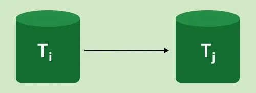
It can be described as a Graph G(V, E) with vertices V = "V1, V2, V3,..., Vn" and directed edges E = "E1, E2, E3,..., En". One of the two operations—READ or WRITE—performed by a certain transaction is contained in the collection of edges. Where Ti -> Tj, means Transaction-Ti is either performing read or write before the transaction-Tj.

Types of Serializability

There are two ways to check whether any non-serial schedule is serializable.

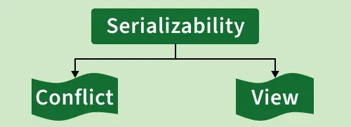
Types of Serializability - Conflict & View

1. Conflict serializability

Conflict serializability ensures database consistency by checking if a non-serial schedule can be rearranged into a serial order by swapping non-conflicting operations. It prevents conflicting operations (like read/write on the same data) from executing at the same time.

Conflict Equivalency

For two schedules (S1 and S2) to be conflict equivalent, they must satisfy the following:

• Same Conflicting Operations: The same conflicting operations (e.g., reads and writes on the same data item) must occur in both schedules in the same order. Example: If t1 writes A before t2 in S1, then t1 must also write A before t2 in S2.

• Non-Conflicting Operations: Operations that do not conflict (e.g., reading different data items) should not affect the order of the schedules. Example: If t1 reads B and t2 reads C in S1, then t1 should still read B and t2 should still read C in S2.

• Preserving Transaction Order: The order of conflicting operations should be the same in both schedules to maintain consistency. Example: If t1 writes A and t2 reads A in S1, t2 must read A after t1 in S2.

In simple terms, conflict equivalency ensures that conflicting operations happen in the same order in both schedules, while non-conflicting ones can appear in any order.

2. View Serializability

View serializability ensures that a non-serial schedule results in the same final outcome as a serial schedule, maintaining database consistency.

To further understand view serializability in DBMS, we need to understand the schedules S1 and S2. The two transactions T1 and T2 should be used to establish these two schedules. Each schedule must follow the three transactions in order to retain the equivalent of the transaction. These three circumstances are listed below.

1. Same Transactions: Both schedules must include the same set of transactions.

2. Same Writes: Each data item must be written by the same transaction in both schedules.

3. Same Reads: Each read must read the same value (from the same write) in both schedules.

View Equivalency

Schedules (S1 and S2) must satisfy these two requirements in order to be view equivalent:

1. The same data must be read first in both schedules. Example: If t1 reads A in S1, it must do the same in S2.

2. The same data must be used for the final write. Example: If t1 updates A last in S1, it should do the same in S2.

3. The middle sequence should also match. Example: If t1 reads A and t2 updates A in S1, the same order should occur in S2.

Example: We have a schedule "S" with two concurrently running transactions, "t1" and "t2."

Schedule S:

Transaction-1 (t1)	Transaction-2 (t2)
R(a)
W(a)
	R(a)
	W(a)
R(b)
W(b)
	R(b)
	W(b)

By switching between both transactions' mid-read-write operations, let's create its view equivalent schedule (S').

Schedule S':

Transaction-1 (t1)	Transaction-2 (t2)
R(a)
W(a)
R(b)
W(b)
	R(a)
	W(a)
	R(b)
	W(b)

Benefits of Serializability

• Predictable Execution: Transactions behave consistently without surprises—no data loss or corruption.

• Easier Debugging: Each transaction runs independently, making errors easier to trace and fix.

• Lower Costs: Reduces need for complex hardware and can cut down development costs.

• Better Performance: Optimized, consistent execution can sometimes outperform non-serial schedules.

---

b) Concurrency Control — Problems

n a Database Management System (DBMS), Concurrency control is a mechanism in DBMS that allows simultaneous execution of transactions while maintaining ACID properties - Atomicity, Consistency, Isolation and Durability. It maintains the integrity, accuracy and reliability of data when multiple users or processes perform read/write operations concurrently. It helps manage issues like:

• Conflicting operations on shared data

• Inconsistent database states

• Lost or incorrect updates

Note: By implementing concurrency control techniques such as locking or timestamp ordering, DBMS ensures that transactions are executed safely and independently, even when they overlap in time.

Need of Concurrency Control

Concurrency control is essential to:

• Prevent conflicts between simultaneous transactions.

• Maintain data consistency and accuracy in multi-user environments.

• Avoid problems such as dirty reads, lost updates and inconsistent reads.

Example:

• Without concurrency control: Two users update the same record simultaneously and one update overwrites the other.

• With concurrency control: The DBMS uses locks or timestamps to ensure updates occur sequentially and data remains correct.

Concurrency Problems in DBMS

When multiple transactions execute concurrently, several problems may occur:

• Dirty Read: A transaction reads uncommitted data from another transaction that may later roll back.

• Lost Update: Two transactions update the same data and one update overwrites the other.

• Inconsistent Read: A transaction reads the same data multiple times and the data changes in between reads.

Concurrency Control Protocols

Concurrency control protocols define rules to ensure correct and consistent execution of transactions. The main protocols are:

1. Lock-Based Concurrency Control: Uses locks to restrict access to data items during a transaction. Common types include shared locks (read) and exclusive locks (write). Ensures serializability and prevents conflicts. Example: Two-Phase Locking (2PL) guarantees that once a transaction releases a lock, it cannot obtain any new locks.

2. Timestamp-Based Concurrency Control: Each transaction is assigned a timestamp. The DBMS uses these timestamps to order transactions and prevent conflicts based on their start time

Types of Lock-Based Protocols

1. Simplistic Lock Protocol

It is the simplest method for locking data during a transaction. Simple lock-based protocols enable all transactions to obtain a lock on the data before inserting, deleting, or updating it. It will unlock the data item once the transaction is completed.

Example: Consider a database with a single data item X = 10.

Transactions:

• T1: Wants to read and update X.

• T2: Wants to read X.

Steps:

1. T1 requests an exclusive lock on X to update its value. The lock is granted.

2. T1 reads X = 10 and updates it to X = 20.

3. T2 requests a shared lock on X to read its value. Since T1 is holding an exclusive lock, T2 must wait.

4. T1 completes its operation and releases the lock.

5. T2 now gets the shared lock and reads the updated value X = 20.

This example shows how simplistic lock protocols handle concurrency but do not prevent problems like deadlocks or limits concurrency.

2. Pre-Claiming Lock Protocol

The Pre-Claiming Lock Protocol avoids deadlocks by requiring a transaction to request all needed locks before it starts. It runs only if all locks are granted; otherwise, it waits or rolls back.

Example: Consider two transactions T1 and T2 and two data items, X and Y:

Transaction T1 declares that it needs:

• A write lock on X.

• A read lock on Y.

Since both locks are available, the system grants them. T1 starts execution: It updates X. It reads the value of Y.

While T1 is executing, Transaction T2 declares that it needs: However, since T1 already holds a write lock on X, T2's request is denied. T2 must wait until T1 completes its operations and releases the locks. A read lock on X

Once T1 finishes, it releases the locks on X and Y. The system now grants the read lock on X to T2, allowing it to proceed.
This method is simple but may lead to inefficiency in systems with a high number of transactions.

3. Two-phase locking (2PL)

A transaction is said to follow the Two-Phase Locking protocol if Locking and Unlocking can be done in two phases :

• Growing Phase: New locks on data items may be acquired but none can be released.

• Shrinking Phase: Existing locks may be released but no new locks can be acquired.

4.Strict Two-Phase Locking Protocol Strict Two-Phase Locking requires that in addition to the 2-PL all Exclusive(X) locks held by the transaction be released until after the Transaction Commits.

5. Rigorous Two- Phase Lock Protocol A stricter form of the Two-Phase Locking (2PL) protocol where all locks (both Shared and Exclusive) are held until the transaction commits.

Problem With Simple Locking

Consider the Partial Schedule:

S.No	T1	T2
1	lock-X(B)
2	read(B)
3	B:=B-50
4	write(B)
5		lock-S(A)
6		read(A)
7		lock-S(B)
8	lock-X(A)
9	......	......

1. Deadlock

In the given execution scenario, T1 holds an exclusive lock on B, while T2 holds a shared lock on A. At Statement 7, T2 requests a lock on B, and at Statement 8, T1 requests a lock on A. This situation creates a deadlock, as both transactions are waiting for resources held by the other, preventing either from proceeding with their execution.

2. Starvation

Starvation is also possible if concurrency control manager is badly designed. For example: A transaction may be waiting for an X-lock on an item, while a `sequence of other transactions request and are granted an S-lock on the same item. This may be avoided if the concurrency control manager is properly designed.

---

Type of Timestamp Ordering

Basic Timestamp Ordering

The Basic TO Protocol works by comparing the timestamp of the current transaction with the timestamps on the data items it wants to read/write:

Precedence Graph for TS ordering

• Suppose, if an old transaction Ti has timestamp TS(Ti), a new transaction Tj is assigned timestamp TS(Tj) such that TS(Ti) < TS(Tj).

• The protocol manages concurent execution such that the timestamps determine the serializability order.

• The timestamp ordering protocol ensures that any conflicting read and write operations are executed in timestamp order.

• Whenever some Transaction T tries to issue a R_item(X) or a W_item(X), the Basic TO algorithm compares the timestamp of T with R_TS(X) & W_TS(X) to ensure that the Timestamp order is not violated.

Strict Timestamp Ordering Protocol

The Strict Timestamp Ordering Protocol is an enhanced version that avoids cascading rollbacks by delaying operations until it's safe to execute them.

Key Features

• Strict Execution Order: Transactions must execute in the exact order of their timestamps. Operations are delayed if executing them would violate the timestamp order, ensuring a strict schedule.

• No Cascading Rollbacks: To avoid cascading aborts, a transaction must delay its operations until all conflicting operations of older transactions are either committed or aborted.

• Consistency and Serializability: The protocol ensures conflict-serializable schedules by following strict ordering rules based on transaction timestamps.

Thomas Write Rule

The Thomas Write Rule (TWR) is an extension of the Basic Timestamp Ordering (TO) Protocol used for concurrency control in Database Management Systems (DBMS).

• Developed by: R. H. Thomas (1979)

• Type: Timestamp-based concurrency control

• Goal: Reduce unnecessary rollbacks while maintaining view serializability

Note: It allows higher concurrency by ignoring obsolete writes instead of aborting transactions, as long as doing so doesn’t affect the final database state.

Basic Idea

In the Basic Timestamp Ordering (TO) protocol, if a transaction tries to write an outdated value, it is aborted. However, in the Thomas Write Rule, instead of aborting, the outdated write is ignored, allowing the transaction to continue.`

Notations:

Symbol	Meaning
TS(T)	Timestamp of transaction T
R_TS(X)	Timestamp of the last read on data item X
W_TS(X)	Timestamp of the last write on data item X

Write Operation Conditions in TWR

1. Abort the Transaction:

• If R_TS(X) > TS(T)

• A newer transaction has already read X, so writing now would violate serializability.

• Action: Abort and rollback T.

2. Ignore Outdated Writes (Allow Execution Without Writing):

• If W_TS(X) > TS(T)

• A newer write has already updated X. Writing now is obsolete.

• Action: Ignore the write; continue the transaction.

3. Execute Write Operation (Normal Execution):

• If neither condition above is true

• Action: Execute W_item(X) and update W_TS(X) = TS(T)

---

Advantages of Concurrency Control

1. Reduced Waiting Time: Multiple transactions can proceed simultaneously, reducing idle time.

2. Improved Response Time: Faster access and interaction with the database.

3. Better Resource Utilization: Hardware and database resources are efficiently shared.

4. Increased System Efficiency: Higher throughput and better overall performance.

Disadvantages of Concurrency Control

1. Overhead: Managing locks and timestamps adds system overhead.

2. Deadlocks: Circular waits between transactions can halt progress.

3. Reduced Concurrency: Locking can limit the number of simultaneous transactions.

4. Complexity: Implementation in distributed or large systems can be difficult.

5. Inconsistencies: Rollbacks or long waits may cause temporary data inaccuracy or staleness.

---

End of Notes — Best of luck for your DBMS examination!